


TABLE OF CONTENTS
Time-Series Databases: InfluxDB vs TimescaleDB vs Prometheus for IoT and Monitoring

A temperature sensor on a factory floor records a reading every five seconds. A Kubernetes cluster emits thousands of metrics per minute from every pod, node, and container. A financial trading platform logs every price tick across hundreds of instruments simultaneously. Each of these workloads shares a common structure: a continuous stream of timestamped numerical measurements, arriving at high velocity, queried almost exclusively by time range, and growing indefinitely until a retention policy prunes the oldest records.
This structure, which defines time-series data, behaves so differently from the transactional data that relational databases were designed to handle that storing it in a general-purpose database produces consistently poor results. A relational table that accumulates a billion timestamped sensor readings will see INSERT performance degrade as indexes grow, query performance collapse on range scans without careful partitioning, and storage costs spiral because relational formats do not compress repeated near-identical values efficiently.
Purpose-built time-series databases solve these problems through storage architectures specifically optimized for append-only, time-ordered data: columnar compression that exploits the repetitive nature of time-series values, automatic data partitioning by time range, and query engines that understand time as a first-class dimension rather than an ordinary column. The three platforms that engineers encounter most frequently in IoT and infrastructure monitoring contexts are InfluxDB, TimescaleDB, and Prometheus. Each takes a meaningfully different approach to the time-series problem, and understanding those differences is what enables informed selection for a given workload.
What Makes Time-Series Data Different
Time-series data has four properties that distinguish it from general-purpose transactional data and that shape every architectural decision in a time-series database. First, writes are almost always append-only: new measurements are always more recent than existing ones, so writes go to the end of the time range rather than updating arbitrary rows. Second, queries are almost always range-based: the most common query pattern is retrieve all measurements for sensor X between time T1 and time T2, which maps naturally to sequential scans over contiguous time ranges. Third, data volume is enormous: a single IoT deployment with one thousand sensors at one-second resolution generates 86.4 million data points per day. Fourth, recent data is accessed far more frequently than old data, which enables tiered storage and aggressive compression of historical records.
These properties allow time-series databases to make architectural trade-offs that general-purpose databases cannot. They can optimize storage layout for sequential writes at the cost of random-access update performance, because time-series data is almost never updated after it is written. They can apply delta encoding and run-length compression that exploits the slowly changing nature of most sensor readings. They can enforce automatic data retention and downsampling policies that convert high-resolution historical data into lower-resolution aggregates, keeping storage costs bounded even as the data volume grows without limit.
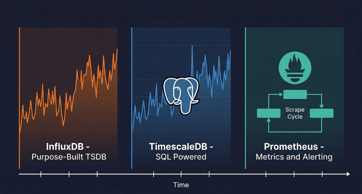
InfluxDB: The Purpose-Built Time-Series Platform
Architecture and Data Model
InfluxDB was designed from the ground up to store and query time-series data. Its data model organizes measurements into a structure that is conceptually similar to a relational table but optimized specifically for time-series access patterns. A measurement is the equivalent of a table name. Tags are indexed metadata fields that identify the source of the measurement: device ID, location, sensor type. Fields are the actual numerical or string values being recorded. Every record carries a timestamp. This four-component model, measurement plus tags plus fields plus timestamp, is how InfluxDB stores every data point.
InfluxDB’s storage engine, TSM (Time-Structured Merge Tree), is a variant of the LSM (Log-Structured Merge Tree) architecture adapted for time-series characteristics. Write-ahead logs accept incoming data points at high throughput. Background compaction merges and compresses data from the write-ahead log into TSM files organized by time range. Compression algorithms exploit time-series patterns aggressively: timestamps are delta-encoded (storing the difference between consecutive timestamps rather than full values), and float values use a variant of the XOR compression algorithm that achieves very high compression ratios on slowly changing sensor readings.
InfluxDB 3.0, released as the current major version, replaces the TSM storage engine with Apache Parquet files stored in object storage (S3 or compatible). This architectural shift separates compute from storage, eliminates the write-ahead log bottleneck that limited InfluxDB 2.x write throughput, and reduces storage costs by an order of magnitude compared to the local disk storage of previous versions. The query layer uses Apache Arrow Flight SQL and DataFusion, the same columnar query engine used by several other modern data platforms, enabling standard SQL alongside InfluxDB’s proprietary Flux query language.
Flux and SQL Query Languages
InfluxDB supports two query languages. Flux is a functional data scripting language developed by InfluxData that treats every query as a pipeline of operations: from() selects a measurement, |> range() filters by time window, |> filter() applies predicate filters, |> aggregateWindow() applies windowed aggregations. Flux is expressive for time-series specific operations like moving averages, derivative calculations, and cross-measurement joins, but its syntax is unfamiliar to engineers accustomed to SQL and has a steeper learning curve for simple queries.
InfluxDB 3.0 adds full SQL support through the Apache DataFusion engine, allowing engineers to query InfluxDB using standard SELECT statements with time-range predicates. This reduces the barrier to adoption significantly for teams that do not want to learn Flux, and it makes InfluxDB compatible with the broader ecosystem of SQL-based tools: dbt models, Grafana data source plugins that expect SQL, and business intelligence platforms that speak standard SQL dialects.
TimescaleDB: PostgreSQL Extended for Time-Series
The Extension Architecture
TimescaleDB is not a standalone database. It is a PostgreSQL extension that adds time-series optimizations to a standard PostgreSQL instance. This architectural decision is both its most distinctive feature and the source of its most significant advantage: every capability, tool, driver, ORM, and ecosystem component that works with PostgreSQL works with TimescaleDB without modification. An application already running on PostgreSQL can activate TimescaleDB by installing the extension and converting time-series tables to hypertables, with no application code changes required beyond that.
The hypertable is TimescaleDB’s core abstraction. From the application perspective, a hypertable behaves exactly like a PostgreSQL table. Queries use standard SQL. Indexes are defined with standard CREATE INDEX syntax. JOINs between hypertables and regular PostgreSQL tables work as expected. Behind the scenes, TimescaleDB automatically partitions the hypertable into chunks based on time range, where each chunk is a standard PostgreSQL table covering a configured time interval. When a query arrives with a time range filter, the query planner performs chunk exclusion: it identifies which chunks overlap the requested time range and scans only those chunks, ignoring all others entirely.
Continuous Aggregates and Compression
TimescaleDB’s continuous aggregates are materialized views that are automatically refreshed as new data arrives. A continuous aggregate defined over a temperature hypertable might compute the hourly average, minimum, and maximum temperature for each sensor. As new readings arrive, TimescaleDB incrementally updates the continuous aggregate rather than recomputing the entire view from scratch. Queries against the continuous aggregate return pre-computed results in milliseconds even on datasets with billions of raw records.
Native compression in TimescaleDB applies columnar compression to older chunks based on a configurable age threshold. A chunk that has not been written to in 24 hours is compressed by rewriting it in a column-oriented format with delta-delta encoding for timestamps and for-loop encoding for integer sequences. Compression ratios of 90 to 97 percent are common for typical IoT datasets, reducing a one-terabyte uncompressed hypertable to 30 to 100 gigabytes of compressed storage while remaining directly queryable through standard SQL without decompression overhead at the query layer.
Prometheus: The Monitoring-Native Metrics System
Pull-Based Architecture and the Prometheus Data Model
Prometheus is a monitoring and alerting system, not a general-purpose time-series database. This distinction matters because Prometheus makes architectural choices that are optimal for infrastructure monitoring but inappropriate for IoT sensor archival or business metrics storage. Understanding what Prometheus was designed for is the prerequisite to using it correctly and to knowing when a different time-series database is needed instead.
Prometheus uses a pull-based collection model. Rather than receiving data that applications push to it, Prometheus periodically scrapes HTTP endpoints that applications expose. Each scrape collects the current value of every metric that the target exposes at that moment. This pull model gives Prometheus control over collection rate and makes it easy to detect when a target has gone offline: a target that fails to respond to a scrape is immediately visible as a collection gap. The trade-off is that Prometheus cannot collect data at sub-second granularity without operational complexity, because scrape intervals are configured globally per scrape job rather than per metric.
The Prometheus data model is dimensional: every metric is identified by a metric name and a set of key-value label pairs. A metric measuring HTTP request duration might be named http_request_duration_seconds with labels for method, status code, and handler path. The combination of metric name and label set uniquely identifies a time series. Prometheus stores each unique label combination as an independent time series, which produces excellent query performance for label-filtered queries but can create a label cardinality problem when labels with high-cardinality values like user IDs or request IDs are used inappropriately.
PromQL and the Alerting Ecosystem
PromQL is Prometheus’s query language, designed specifically for real-time metrics queries and alerting rules. It operates on instant vectors (the current value of a set of time series), range vectors (the values of a set of time series over a time window), and scalars. PromQL’s time-series specific functions like rate(), irate(), histogram_quantile(), and increase() express common monitoring calculations concisely. The rate() function calculates the per-second average rate of increase of a counter over a time window, which is the standard way to express request throughput, error rate, and similar throughput metrics from Prometheus counters.
Prometheus integrates natively with Alertmanager, which handles alert routing, grouping, deduplication, and notification delivery. Alert rules defined in PromQL evaluate continuously against current metric values. When a rule’s condition is satisfied for a configured duration, Prometheus fires an alert to Alertmanager, which routes it to the appropriate notification channel: PagerDuty, Slack, email, OpsGenie, or any other supported receiver. This tight integration between metrics collection, query, and alerting makes Prometheus the standard infrastructure monitoring solution for Kubernetes environments, where it is the first-class monitoring backend for the kube-prometheus-stack Helm chart.
Build Your IoT and Monitoring Data Infrastructure with Askan
Head-to-Head Comparison
| Dimension | InfluxDB 3.0 | TimescaleDB |
|---|---|---|
| Data model | Measurement, tags, fields, timestamp | Standard PostgreSQL tables (hypertables) |
| Query language | Flux and SQL (via DataFusion) | Full PostgreSQL SQL |
| Storage engine | Apache Parquet on object storage | Columnar-compressed PostgreSQL chunks |
| ACID transactions | Limited (append-optimized) | Full ACID via PostgreSQL |
| JOINs with relational data | Limited cross-measurement joins | Full SQL JOINs with any PostgreSQL table |
| Ecosystem compatibility | InfluxDB-native clients | Any PostgreSQL driver, ORM, or tool |
| Managed cloud option | InfluxDB Cloud | Timescale Cloud |
| Dimension | Prometheus | InfluxDB / TimescaleDB |
|---|---|---|
| Primary use case | Infrastructure and application monitoring | IoT, business metrics, long-term archival |
| Collection model | Pull (scrapes targets on schedule) | Push (applications write to the database) |
| Retention | Short-term (15 days default; configurable) | Long-term archival with tiered compression |
| Query language | PromQL | Flux / SQL / standard SQL |
| Alerting | Native via Alertmanager | Requires external alerting tool |
| Cardinality handling | Sensitive to high label cardinality | Better handling of high-cardinality tags |
| Kubernetes native | First-class with kube-prometheus-stack | Requires separate integration |
When to Use Each Database
InfluxDB Is the Right Choice When
InfluxDB is the natural fit for IoT data collection platforms where the primary requirement is high write throughput from a large number of sensors or devices. Its schema-less tag model allows new devices and sensor types to be onboarded without schema migrations, which is a practical advantage in IoT deployments where the device fleet evolves frequently. The InfluxDB Cloud Serverless tier eliminates cluster management entirely, making it accessible for teams that want a dedicated time-series store without infrastructure overhead.
InfluxDB works particularly well for use cases where the time-series data is relatively self-contained and does not need to be joined frequently against relational operational data. Industrial sensor monitoring, environmental tracking, energy consumption logging, and fleet telemetry are all workloads where InfluxDB’s data model and compression deliver strong results without the PostgreSQL ecosystem overhead that TimescaleDB carries.
TimescaleDB Is the Right Choice When
TimescaleDB is the strongest choice when time-series data needs to coexist with relational data in the same database and be queried together using standard SQL. A SaaS platform that stores per-customer usage metrics alongside customer account records, subscription tiers, and billing data can run both in a single TimescaleDB instance. Joining usage metrics to customer dimensions in a single query is straightforward SQL. With InfluxDB or Prometheus, the same join requires either application-level aggregation across two databases or a data pipeline that copies one dataset into the other.
The existing PostgreSQL investment that most engineering teams already have, in terms of expertise, tooling, operational runbooks, and backup procedures, transfers directly to TimescaleDB. Teams that understand how to tune PostgreSQL, configure pg_bouncer, set up streaming replication, and run EXPLAIN ANALYZE can apply all of that knowledge to TimescaleDB without a separate learning curve. This operational familiarity is a significant real-world advantage that pure time-series databases cannot match for teams already running PostgreSQL in production.
For teams evaluating TimescaleDB alongside the broader PostgreSQL ecosystem, the March 23 article on PostgreSQL vs MySQL vs MongoDB database selection covers the foundational PostgreSQL architectural strengths that TimescaleDB inherits.
Prometheus Is the Right Choice When
Prometheus is the right choice when the primary requirement is infrastructure and application monitoring with alerting, particularly in Kubernetes environments. Its native integration with the Kubernetes API server, kube-state-metrics, node-exporter, and every major cloud-native application that exposes a /metrics endpoint makes it the zero-configuration monitoring baseline for cloud-native architectures. The kube-prometheus-stack Helm chart deploys Prometheus, Alertmanager, and Grafana in minutes with pre-configured dashboards and alert rules that cover the most common Kubernetes health conditions.
Prometheus is not the right choice for long-term metrics retention, high-cardinality data, or IoT ingestion workloads. Its local storage is not designed for multi-year archival. Its sensitivity to label cardinality makes it inappropriate for metrics where the label set includes user IDs, session IDs, or request IDs. For these requirements, Prometheus is typically used as a short-term collection and alerting layer that forwards metrics to a long-term backend.
Long-Term Storage: Extending Prometheus with Remote Write
Prometheus’s remote write protocol allows it to forward scraped metrics to a compatible long-term storage backend in real time. This creates a common architecture pattern for large-scale monitoring: Prometheus handles local collection, alerting, and short-term querying while a remote backend handles long-term retention, high-cardinality storage, and global aggregation across multiple Prometheus instances.
Thanos and Grafana Mimir are the two dominant open-source solutions for scaling Prometheus to multi-cluster, long-term retention environments. Thanos extends Prometheus by adding a sidecar that uploads completed TSDB blocks to object storage (S3 or GCS), a query layer that federates queries across multiple Prometheus instances and the object storage backend, and a compactor that downsamples old blocks to reduce long-term storage costs. Mimir is a horizontally scalable, multi-tenant Prometheus backend that accepts remote write from multiple Prometheus instances and provides a PromQL-compatible query API across the unified metric store.
VictoriaMetrics is an alternative that many teams choose over Thanos and Mimir for its simpler operational model. It provides a single-binary deployment that accepts Prometheus remote write, exposes a MetricsQL query endpoint compatible with PromQL, and delivers higher write throughput and better compression than Prometheus’s native TSDB on equivalent hardware. For teams that want Prometheus-compatible long-term storage without the operational complexity of Thanos or Mimir, VictoriaMetrics is frequently the most pragmatic choice.
Build Your IoT and Monitoring Data Infrastructure with Askan
Grafana: The Visualization Layer Across All Three
Grafana is the dominant open-source visualization and dashboarding platform for time-series data, and it provides first-class data source plugins for all three databases covered in this article. A Grafana instance connected to InfluxDB, TimescaleDB, and Prometheus simultaneously can display metrics from all three on a unified dashboard, allowing engineers to correlate IoT sensor data, business metrics, and infrastructure health in a single view without data duplication.
Grafana Alerting, introduced as a unified alerting system in Grafana 9, consolidates alert rules from Prometheus Alertmanager, InfluxDB alerts, and TimescaleDB query-based alerts into a single interface with unified routing, silencing, and notification management. For organizations running multiple time-series backends, Grafana Alerting removes the need to manage separate alerting configurations for each backend.
The observability stack design principles, including how metrics fit alongside logs and distributed traces in a comprehensive monitoring architecture, are covered in the March 18 article on building observable systems. Time-series databases are the storage layer for the metrics pillar of that observability stack.
IoT-Specific Considerations
IoT deployments introduce constraints that standard server-side monitoring workloads do not face. Devices may operate on intermittent network connections, sending bursts of buffered readings when connectivity is restored rather than a steady stream. They may produce readings at irregular intervals rather than fixed scrape cadences. They may fail silently, stopping transmission without any error notification, requiring the monitoring system to detect data gaps rather than explicit failure signals.
InfluxDB handles bursty IoT writes well because its write path is designed for high-throughput batch ingestion. Devices can buffer readings locally and flush batches to InfluxDB when connectivity is restored without the database experiencing performance degradation from the burst. TimescaleDB handles the same pattern through PostgreSQL’s standard INSERT batching, with the additional option of using COPY for bulk loads of buffered historical readings.
The MQTT protocol is the standard message transport for IoT device telemetry. Devices publish sensor readings to an MQTT broker such as Eclipse Mosquitto or EMQX. A bridge service subscribes to MQTT topics and writes the incoming readings to the time-series database. Telegraf, InfluxData’s open-source data collection agent, provides a native MQTT consumer input plugin that reads from MQTT topics and writes to InfluxDB without custom bridge code. For TimescaleDB, the same Telegraf agent supports a PostgreSQL output plugin that writes metrics directly to TimescaleDB hypertables.
Data Retention and Downsampling Strategies
Long-running time-series deployments without a retention and downsampling strategy accumulate unbounded data volumes that eventually make both storage costs and query performance unmanageable. The standard approach is a tiered retention policy that keeps high-resolution recent data, downsampled medium-resolution data for the past year, and further downsampled low-resolution data for multi-year historical analysis.
| Database | Retention Mechanism | Downsampling Mechanism |
|---|---|---|
| InfluxDB | Retention policies per bucket; automatic deletion after TTL | Flux tasks or scheduled InfluxDB tasks writing to separate buckets |
| TimescaleDB | Retention policy via add_retention_policy(); automatic chunk dropping | Continuous aggregates with longer time buckets; refresh policy |
| Prometheus | Global retention via –storage.tsdb.retention.time flag | Thanos or Mimir compactor downsampling; recording rules for pre-aggregation |
TimescaleDB’s continuous aggregate downsampling is particularly elegant in practice. A single SQL query defines both the aggregation logic and the time bucket size. TimescaleDB computes and stores the aggregated results incrementally and serves queries against the continuous aggregate rather than the raw hypertable when the time bucket aligns with the query window. This means a query for monthly average temperature automatically reads from the monthly continuous aggregate rather than scanning billions of raw readings, with no application code required to route the query to the right resolution tier.
Selecting the Right Database for Your Workload
| Workload | Best Choice | Key Reason |
|---|---|---|
| IoT sensor ingestion at high volume | InfluxDB 3.0 | Purpose-built ingestion, schema-less tags, object storage backend |
| Infrastructure and Kubernetes monitoring | Prometheus + Thanos/Mimir | Pull model, kube-prometheus-stack, native alerting |
| Time-series alongside relational data | TimescaleDB | Full SQL JOINs, PostgreSQL ecosystem, single database |
| Long-term Prometheus archival | VictoriaMetrics or Thanos | Remote write compatible, lower cost, better compression |
| Business metrics with SQL analysts | TimescaleDB | Standard SQL, BI tool compatible, continuous aggregates |
| Multi-cloud metrics federation | Grafana Mimir | Multi-tenant, globally queryable Prometheus-compatible store |
| Edge device with local storage | InfluxDB Edge or TimescaleDB | Both support embedded single-node deployment |
The database architecture decisions covered in this article sit within the broader Database Architecture and Performance theme that has run through this week’s articles on the Askan Technologies blog. The March 24 article on database scaling strategies covers the horizontal and vertical scaling patterns that time-series databases at large scale require. The March 26 article on data warehouse vs data lake vs data lakehouse covers how time-series metrics integrate into the broader analytics infrastructure stack when business intelligence teams need access to operational metrics alongside transactional data.
The full-stack engineering practice at Askan Technologies covers IoT platform architecture, time-series database selection and implementation, Prometheus and Grafana stack deployment, and long-term metrics retention pipeline design for engineering teams building monitoring-heavy applications across industries.
Build Your IoT and Monitoring Data Infrastructure with Askan
Most popular pages
-
On-Call Culture Done Right: How to Reduce Alert Fatigue Without Reducing Reliability
Engineering teams in high-growth organisations face a paradox that rarely gets spoken about openly. The same monitoring and alerting systems built to protect uptime...
-
AI-Assisted Code Review: What Works, What Does Not, and How Teams Are Adapting
AI tools have moved quickly from experimental additions into everyday developer workflows. Code review, which has always been one of the most time-consuming parts...
-
Async Communication in Engineering Teams: When Fewer Meetings Produce Better Code
There is a version of the engineering day that many developers know well. The calendar is split into one-hour blocks. Stand-ups run long. Syncs...
On-Call Culture Done Right: How to Reduce Alert Fatigue Without Reducing Reliability
Engineering teams in high-growth organisations face a paradox that rarely gets spoken about openly. The same monitoring and alerting systems built to protect uptime...
AI-Assisted Code Review: What Works, What Does Not, and How Teams Are Adapting
AI tools have moved quickly from experimental additions into everyday developer workflows. Code review, which has always been one of the most time-consuming parts...
Async Communication in Engineering Teams: When Fewer Meetings Produce Better Code
There is a version of the engineering day that many developers know well. The calendar is split into one-hour blocks. Stand-ups run long. Syncs...