


TABLE OF CONTENTS
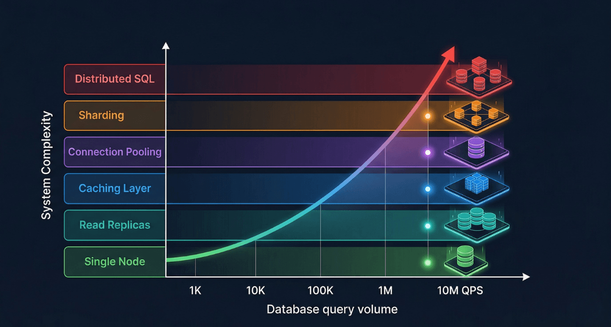
Database Scaling Strategies: From 1K to 10M Queries Per Second

Most databases start their lives handling a few hundred queries per second against a schema designed in a weekend. The first thousand users arrive and nothing breaks. The first ten thousand users arrive and a few slow queries surface. By the time a hundred thousand concurrent users are active, the database that was fine last month has become the most expensive and fragile component in the entire system.
Database scaling is not a single technique applied once. It is a progression of architectural decisions, each one extending the ceiling of what your database can handle before the next constraint emerges. Engineers who understand the full scaling progression make better decisions at each stage because they know what is coming next. They design schemas and access patterns that do not close off future scaling options. They add complexity only when the current tier has genuinely been exhausted, rather than prematurely over-engineering.
This guide traces the full scaling journey from a single database node handling one thousand queries per second to a distributed system capable of sustaining ten million queries per second. Each tier is covered in depth: what it solves, how to implement it, what it costs, and when to move to the next level.
Understanding Query Volume and What QPS Actually Measures
Queries per second is a deceptively simple metric. A single page load in a modern web application can generate dozens of database queries: session validation, user profile retrieval, content queries, recommendation lookups, ad targeting, and analytics events. An application serving fifty thousand page views per hour at forty queries per page load is issuing more than half a million database queries per minute, roughly nine thousand per second, from a traffic volume that sounds modest.
The nature of those queries matters as much as the count. A database serving nine thousand simple primary key lookups per second is under very different stress than one serving nine thousand complex analytical queries with table scans. Query complexity, data volume per query, locking behavior, and write-to-read ratio all determine how a database behaves under load in ways that raw QPS does not capture.
| QPS Range | Typical Application Stage | Primary Bottleneck |
|---|---|---|
| 1 to 5K QPS | Early-stage product, up to 50K daily active users |
None: single well-configured node handles this tier comfortably |
| 5 to 50K QPS | Growth-stage product, 50K to 500K daily active users |
Read capacity of a single node; slow query accumulation |
| 50 to 500K QPS | Scaled product, 500K to 5M daily active users |
Read replica fan-out, connection management, cache hit rate |
| 500K to 5M QPS | Large-scale platform, millions of daily active users |
Write throughput, sharding decisions, hot partition avoidance |
| 5M to 10M+ QPS | Hyperscale systems, global distributed deployment |
Cross-shard consistency, network latency, global data distribution |
Tier 1: Optimizing the Single Node (1K to 10K QPS)
Why Start Here
The first response to a slow database should never be adding hardware or architectural complexity. The majority of performance problems at the 1K to 10K QPS range are caused by missing indexes, poorly written queries, suboptimal schema design, or misconfigured server parameters. Adding a read replica to a database that has a full table scan executing on every page load accelerates the full table scan without solving the underlying problem.
A single PostgreSQL or MySQL instance on modern hardware, properly configured, can sustain 50K to 100K simple read queries per second. If you are experiencing performance problems at 5K QPS, the problem is almost certainly not hardware capacity. It is something in the application or schema that is wasting the capacity you already have.
Query Analysis and Slow Query Identification
PostgreSQL’s pg_stat_statements extension tracks execution statistics for every distinct query pattern: total execution count, mean execution time, total time consumed, rows returned, and buffer cache hit rate. Querying pg_stat_statements ordered by total execution time identifies the queries that consume the most cumulative database time, which is a more actionable metric than mean execution time alone. A query that runs in 100 milliseconds but executes ten thousand times per minute contributes more to total database load than a query that takes two seconds but runs once per hour.
MySQL’s performance_schema.events_statements_summary_by_digest table provides equivalent statistics. The slow query log, enabled by setting long_query_time to a threshold like 0.1 seconds, captures full query text and execution details for queries that exceed the threshold, including queries that are slow due to lock waits rather than computational cost.
Index Optimization at the Single-Node Stage
EXPLAIN ANALYZE in PostgreSQL and EXPLAIN FORMAT=JSON in MySQL reveal the query execution plan: which indexes are used, how many rows are estimated vs. actually scanned, and where nested loop joins are producing Cartesian-product-scale work. A query plan showing Seq Scan on a table with millions of rows is the clearest possible signal that an index is missing or that the query planner is not using an available index due to stale table statistics.
Partial indexes eliminate index overhead for low-selectivity columns. An index on a status column with three values (pending, active, completed) in a table of ten million rows where 95% of rows have status active and only 5% are pending is poorly selective for queries filtering on active. A partial index created with WHERE status = ‘pending’ indexes only the 500,000 pending rows, producing a compact index that lookups of pending records use efficiently while not wasting space on active rows that are rarely filtered in isolation.
| Index Optimization Technique | When to Apply |
|---|---|
| Composite index (covering index) | Queries filtering and sorting on multiple columns in a consistent pattern |
| Partial index | Queries that always filter to a high-selectivity subset of rows |
| Index-only scan (include columns) | Queries that SELECT only indexed columns, avoiding heap access entirely |
| Expression index | Queries filtering on a function of a column: lower(email), date_trunc(‘day’, created_at) |
| BRIN index | Append-only tables where column values increase monotonically with row insertion order |
Server Configuration Tuning
Default PostgreSQL configuration is intentionally conservative, designed to run safely on a 256 MB virtual machine from 2005. A production server with 32 GB of RAM running PostgreSQL with default settings leaves the majority of available memory unused by the database engine. Three parameters produce the largest gains with the least risk.
| Parameter | Recommended Starting Value (32 GB RAM server) |
|---|---|
| shared_buffers | 8 GB (25% of total RAM) |
| effective_cache_size | 24 GB (75% of total RAM, advisory only) |
| work_mem | 64 MB (per sort/hash operation, monitor for OOM risk) |
| max_connections | 200 with PgBouncer in front limiting actual connections |
| checkpoint_completion_target | 0.9 (spread checkpoint writes to reduce I/O spikes) |
| wal_buffers | 64 MB (reduce WAL write latency under write bursts) |
MySQL’s key configuration parameters follow a similar pattern. innodb_buffer_pool_size should be set to 70 to 80 percent of available RAM on a dedicated database server. innodb_log_file_size controls the size of the InnoDB redo log, which directly affects write throughput under heavy insert and update workloads. Setting it to 1 GB or larger reduces the frequency of checkpoint flushes and improves sustained write throughput significantly compared to the default 48 MB.
Tier 2: Read Replicas (10K to 100K QPS)
The Read Replica Architecture
Most web applications have a read-to-write ratio between 5:1 and 20:1. Users browse, search, and view content far more frequently than they create, update, or delete it. This asymmetry means that scaling read capacity independently from write capacity produces the highest throughput-per-dollar improvement at the 10K to 100K QPS range.
A read replica is a continuously synchronized copy of the primary database that serves read queries while the primary handles all writes. PostgreSQL implements replication through Write-Ahead Log (WAL) shipping: the primary writes every change to its WAL and streams those WAL records to replicas, which apply them in order, keeping the replica’s data state close to the primary with a lag that is typically under one second on well-connected servers.
Replication Lag and Read Consistency
The most important operational characteristic of read replicas is replication lag. Replica data is always slightly behind the primary because WAL records must travel over the network and be applied before the replica can serve the updated data. For most read workloads this is acceptable: a user’s activity feed that reflects writes from two seconds ago is functionally correct for the user experience.
The failure mode is read-after-write inconsistency: a user submits a form, the write goes to the primary, the page reload reads from a replica that has not yet applied the write, and the user sees their own change missing. Applications must identify which read operations require consistency with recent writes and route those specific queries to the primary rather than replicas.
| Consistency Strategy | Implementation |
|---|---|
| Route reads after writes to primary | Track writes per user session, route subsequent reads to primary for a short window |
| Synchronous replication for critical reads | PostgreSQL synchronous_standby_names: replica acknowledges before primary commits |
| Read your own writes from primary only | Simpler: route all reads for a user session to the primary immediately after any write in that session |
| Replica lag monitoring | Track pg_stat_replication.write_lag and alert when lag exceeds 1 second |
AWS Aurora: Eliminating Replication Lag
AWS Aurora’s storage architecture separates compute and storage in a way that eliminates traditional replication lag. All Aurora instances in a cluster, both the primary writer and up to 15 read replicas, share the same underlying distributed storage volume. When the primary writes data, the storage layer propagates it immediately. Replicas do not need to receive and apply WAL records; they read from the same storage that the primary just wrote to. Replica lag in Aurora is typically under 10 milliseconds, compared to hundreds of milliseconds possible with traditional streaming replication under write bursts.
Aurora also supports auto-scaling read replicas through Aurora Auto Scaling, which adds replicas when connection count or CPU utilization on existing replicas exceeds a threshold, and removes them when load drops. This elasticity makes Aurora a strong choice for applications with unpredictable read traffic spikes.
Hit a Database Performance Ceiling? Let Us Help.
Tier 3: Caching Layers (50K to 500K QPS)
Why Caching Multiplies Database Capacity
A cache hit is a database query that never reaches the database. At the 50K to 500K QPS range, the most effective scaling strategy is reducing the number of queries that reach the database at all by serving frequently requested data from an in-memory cache. If 80% of your database reads request data that changes less often than once per minute, and that data can be cached for 60 seconds, you have eliminated 80% of your read query load with a single architectural addition.
Redis and Memcached are the two dominant in-memory caching platforms. Redis is the more capable of the two: it supports rich data structures (strings, hashes, lists, sorted sets, streams), built-in data expiration with TTL, pub/sub messaging, Lua scripting, and optional persistence. Memcached is simpler and slightly faster for pure string key-value operations, but its lack of data structures and persistence limits its applicability beyond pure caching workloads. For most production systems, Redis handles both caching and session storage, consolidating two infrastructure components into one.
Caching Strategy Selection
| Strategy | How It Works | Best For |
|---|---|---|
| Cache-aside (lazy loading) |
Application checks cache first; on miss, loads from DB and writes to cache |
Read-heavy data with unpredictable access patterns |
| Write-through | Every write goes to DB and cache simultaneously;cache always has fresh data |
Data where stale reads are unacceptable |
| Write-behind (write-back) |
Write goes to cache first, flushed to DB asynchronously |
High-write workloads where some data loss is tolerable |
| Read-through | Cache fetches from DB automatically on miss; app only talks to cache |
Simplifies application code; works well with ORM-level caching |
| Refresh-ahead | Cache proactively refreshes entriesbefore they expire based on access patterns |
Hot data with predictable access and expensive recalculation |
Cache Key Design and Invalidation
Cache key design determines both hit rate and correctness. A key that is too coarse, such as caching an entire user’s order history under a single key, invalidates the entire cached object when any single order changes, producing unnecessary cache misses and database load. A key that is too granular, one key per order line item, produces excessive cache memory overhead and complex invalidation logic.
The most reliable invalidation strategies are TTL-based expiry for data where brief staleness is acceptable, and event-driven invalidation for data where stale reads produce visible inconsistencies. Event-driven invalidation publishes a cache invalidation message when the underlying data changes, and all application instances that hold the cached value delete it on receiving the event. This approach requires a reliable event bus but produces correct cache state without requiring the application to track every cache key that might be affected by a given write.
| Invalidation Method | Trade-offs |
|---|---|
| TTL expiry (time-based) | Simple to implement; brief staleness window is acceptable for most use cases |
| Write-through invalidation | Cache is updated synchronously on write; consistent but adds write latency |
| Event-driven delete | Reliable correctness; requires event bus infrastructure |
| Cache versioning | Append version number to cache key; old keys expire naturally, no explicit delete needed |
Redis Cluster for Cache Scaling
A single Redis instance handles hundreds of thousands of operations per second and stores tens of gigabytes of data. For applications that exceed single-instance capacity, Redis Cluster distributes data across multiple nodes using consistent hashing. Each node is responsible for a subset of the 16,384 hash slots that Redis Cluster uses to partition keys. Adding nodes redistributes hash slots automatically, scaling cache capacity without application changes.
Redis Sentinel provides high availability for non-cluster deployments by monitoring the primary Redis instance and automatically promoting a replica to primary when the primary fails. AWS ElastiCache and Google Cloud Memorystore provide managed Redis with automatic failover, backup, and scaling, removing the operational burden of managing Redis cluster topology in self-hosted environments.
Tier 4: Connection Pooling (All Tiers Above 10K QPS)
Connection pooling is not a scaling tier in the same sense as replicas or caching, but it is a prerequisite for every higher scaling tier. PostgreSQL’s process-per-connection model means each open database connection consumes memory and system resources whether or not it is actively running a query. At 500 connections, PostgreSQL consumes significant memory just on connection overhead. At 5,000 connections, the overhead can exhaust server memory before query processing begins.
PgBouncer operates as a connection proxy that maintains a small pool of actual database connections and multiplexes many application connections onto them. In transaction pooling mode, a database connection is held for only the duration of a single transaction, then returned to the pool. An application with 2,000 concurrent users might require only 50 actual database connections in PgBouncer transaction mode if each transaction completes in under 50 milliseconds.
| PgBouncer Mode | Connection Held For | Use Case |
|---|---|---|
| Session pooling | Entire client session lifetime | Applications using session-level features (SET LOCAL, advisory locks) |
| Transaction pooling | Single transaction duration only | Standard OLTP workloads, most web applications |
| Statement pooling | Single statement duration | Simple read-only queries; incompatible with multi-statement transactions |
ProxySQL serves the same role for MySQL deployments, with the additional capability of query routing: it can parse incoming SQL and route read queries to replicas and write queries to the primary based on query type, without requiring application-level routing logic. This makes ProxySQL a combined connection pooler and read/write splitter for MySQL architectures.
Hit a Database Performance Ceiling? Let Us Help.
Tier 5: Vertical Scaling and Hardware Optimization
Before sharding, which dramatically increases architectural complexity, vertical scaling of the database server is worth evaluating. Modern cloud instances with 192 GB of RAM and 64 vCPUs can sustain hundreds of thousands of queries per second for read-heavy workloads. If the working dataset, the portion of data frequently accessed, fits entirely in RAM, the operating system buffer cache will satisfy most reads from memory without disk I/O, producing very high throughput from a single node.
The working set principle is fundamental to database performance at scale. A 500 GB database where 95% of production queries access the most recent 20 GB of data (recent orders, active user sessions, current catalog) has an effective working set of 20 GB. A database server with 64 GB of RAM will keep that working set in memory after a brief warmup period, serving the vast majority of reads from RAM at nanosecond access times rather than from disk at millisecond access times.
| Hardware Factor | Scaling Impact |
|---|---|
| RAM (working set fits in memory) | Most impactful single hardware change; eliminates disk I/O for hot data |
| NVMe SSD storage | 10x lower latency than SATA SSD for queries that do require disk I/O |
| CPU core count | Increases parallel query execution capacity and connection handling |
| Network bandwidth | Critical for replication throughput and large result set transfers |
Tier 6: Sharding (500K to 10M QPS)
What Sharding Actually Means
Sharding distributes data across multiple independent database nodes, each holding a subset of the total dataset. Unlike replication where every node holds a full copy of the data, sharding divides the data so that each shard holds a distinct partition. A write to the database goes to exactly one shard. A read that requires data from multiple shards must query multiple shards and aggregate the results at the application or proxy layer.
Sharding solves the write scaling problem that read replicas cannot address. Adding read replicas increases read capacity, but all writes still go to a single primary node. When write throughput saturates the primary’s capacity, no number of read replicas helps. Sharding distributes both reads and writes across multiple nodes, scaling both dimensions simultaneously.
Shard Key Selection: The Most Critical Sharding Decision
The shard key determines how data is distributed across shards. A poor shard key produces hot shards, where one shard receives the majority of traffic while others sit idle, negating the entire scaling benefit. A shard key on a timestamp column in an append-only table sends every new write to the shard covering the most recent time range, creating a write hot spot. A shard key on a low-cardinality status column creates a small number of very large shards with no meaningful distribution.
| Shard Key Characteristic | Effect | Recommendation |
|---|---|---|
| High cardinality (user_id, account_id) |
Even distribution across shards | Strong choice for user-centric data |
| Monotonically increasing (timestamp, auto-increment ID) |
All new writes go to the last shard | Avoid as a standalone shard key |
| Low cardinality (status, country) |
Uneven distribution, few large shards | Never use as a shard key |
| Composite key (region + user_id) |
Combines geographic locality with even distribution |
Good for globally distributed systems |
| Hashed key (hash of user_id) |
Perfectly even mathematical distribution | Best for uniform distribution; sacrifices range query efficiency |
Application-Level Sharding vs. Middleware Sharding
Application-level sharding places the shard routing logic in the application code. The application computes which shard a given record belongs to and opens the appropriate database connection. This approach is transparent and debuggable but couples the application to the sharding topology. Adding a new shard requires modifying the routing logic and rebalancing data across shards.
Middleware sharding uses a proxy layer that intercepts all database queries, applies shard routing logic, and forwards queries to the appropriate shards transparently. Vitess (originally built at YouTube for MySQL) and Citus (PostgreSQL extension) implement middleware sharding with automatic query routing, distributed joins across shards, and online resharding without application changes. Vitess handles cross-shard transactions through two-phase commit and supports horizontal resharding by splitting shards while the system remains online.
| Sharding Solution | Best Fit |
|---|---|
| Vitess (MySQL) | Large MySQL deployments needing horizontal write scaling without application rewrites |
| Citus (PostgreSQL) | PostgreSQL workloads with analytical and transactional queries across distributed data |
| PlanetScale | Managed MySQL-compatible sharding with schema change tooling |
| CockroachDB | PostgreSQL-compatible distributed SQL with automatic sharding and geo-partitioning |
| Application-level sharding | Simple use cases where data partitioning is clean and cross-shard queries are rare |
Cross-Shard Query Challenges
The central trade-off of sharding is that queries requiring data from multiple shards must be executed against each relevant shard and the results merged. A simple user profile lookup by user_id in a user-sharded database hits exactly one shard and performs identically to a single-node query. A query for all users in a specific geographic region, when the sharding key is user_id rather than region, must query all shards and merge the results, consuming resources proportional to the number of shards rather than the size of the result.
Schema design for sharded systems must minimize cross-shard queries by co-locating related data on the same shard. In a user-sharded e-commerce system, a user’s orders, payment methods, and session data should all be stored on the same shard as the user record. This co-location strategy allows queries that span user and order data to execute within a single shard, preserving the performance benefits of sharding for the most common access patterns.
Tier 7: Distributed SQL and Global Distribution (5M to 10M+ QPS)
At the highest traffic tiers, where single-region deployments cannot absorb the full query volume and global user bases require sub-100ms read latency from multiple continents, distributed SQL databases provide a managed solution to the problems that manual sharding requires teams to solve themselves.
CockroachDB and Google Spanner implement distributed SQL that spans multiple nodes and regions while maintaining full ACID compliance across all nodes. They handle automatic data distribution, replication, failover, and distributed transaction coordination internally. The application interacts with a PostgreSQL-compatible interface (CockroachDB) or a Spanner-specific SQL dialect, and the database layer manages all distributed coordination transparently.
| Distributed SQL Option |
Consistency Model | Best Fit |
|---|---|---|
| CockroachDB | Serializable isolation, geo-partitioning | Global PostgreSQL-compatible applications |
| Google Spanner | External consistency (stronger than Serializable) |
Google Cloud-native, global financial systems |
| YugabyteDB | PostgreSQL and Cassandra APIs, tunable consistency |
Hybrid OLTP and analytics workloads |
| TiDB | Snapshot isolation, MySQL-compatible |
Large-scale MySQL migrations to distributed SQL |
The operational simplicity of managed distributed SQL comes at a cost: these systems are more expensive per QPS than self-managed sharded MySQL or PostgreSQL, and their query planners sometimes produce suboptimal plans for complex analytical queries that a carefully tuned single-node PostgreSQL would handle more efficiently. They are the right choice when the operational complexity of managing a manually sharded cluster has become the primary engineering burden, and when global consistency guarantees justify the premium.
Read Query Optimization: Beyond Replicas
Materialized Views
Materialized views precompute and store the results of expensive queries as physical tables that can be queried instantly. A dashboard that aggregates order revenue by product category, date, and region from a table with a billion rows would normally require a multi-second full aggregation query. A materialized view refreshed hourly stores the aggregated result and serves the dashboard query in milliseconds.
PostgreSQL supports materialized views natively with REFRESH MATERIALIZED VIEW CONCURRENTLY, which refreshes the view without locking reads against the stale version. Timescale’s continuous aggregates extend this pattern to time-series data, automatically maintaining pre-aggregated rollups as new time-series data is inserted, eliminating the need to manually schedule refresh jobs.
Query Result Caching at the Database Layer
ProxySQL implements query result caching at the database proxy layer, serving identical queries from in-memory cache without forwarding them to the database at all. Unlike application-level caching, which requires explicit cache management code in every query path, ProxySQL cache operates transparently based on query digest matching. Queries that match a configured digest pattern are served from cache for a configured TTL, then refreshed from the database when the TTL expires.
This approach is most effective for queries that are identical across many requests, such as global configuration lookups, product catalog queries for popular items, and reference data like country codes and currency lists. It is less effective for queries with high-cardinality parameters, such as per-user personalized data, where each query is unique and cache hit rates are low regardless of TTL configuration.
Write Scaling Techniques Short of Full Sharding
Write Batching and Bulk Inserts
Individual INSERT statements carry per-statement overhead: transaction log writes, index updates, and constraint checks executed once per row. A workload that inserts ten thousand rows individually can be ten to fifty times slower than a single bulk insert of the same ten thousand rows. Batching writes into bulk operations reduces overhead by amortizing per-statement costs across many rows in a single transaction.
PostgreSQL’s COPY command is the fastest mechanism for bulk data loading, operating at the storage level rather than through the SQL parser. For real-time event ingestion where rows arrive continuously, a write buffer that accumulates events for 100 milliseconds and then flushes as a bulk insert produces dramatically higher sustained write throughput than row-by-row insertion while adding only 100 milliseconds of write latency.
Table Partitioning for Write and Query Performance
Table partitioning divides a large logical table into smaller physical partitions based on a partition key, typically a time range for time-series data or a range/list of values for categorical data. The database query planner performs partition pruning: queries that filter on the partition key skip partitions that cannot contain matching rows, reducing the effective scan scope to only the relevant partitions.
For write performance, partitioning enables partition-specific index maintenance and vacuum operations. In PostgreSQL, autovacuum operates on individual partitions rather than the entire table, keeping dead row cleanup efficient as the table grows. Old partitions containing historical data can be detached and archived to cold storage without locking the live partitions, keeping the active dataset compact and the working set small.
| Partition Type | Partition Key | Best Use Case |
|---|---|---|
| Range partitioning | Date or timestamp column | Time-series data: logs, events, metrics, orders |
| List partitioning | Categorical column: region, status, tenant_id |
Multi-tenant data or geographic data isolation |
| Hash partitioning | Any high-cardinality column | Even distribution without range query requirements |
Putting It Together: The Scaling Decision Ladder
Each scaling tier introduces complexity that should only be accepted when the previous tier has been genuinely exhausted. The following sequence reflects the order in which scaling actions deliver the highest return on engineering investment.
| Step | Action |
|---|---|
| 1. Identify slow queries | pg_stat_statements / slow query log, target top 10 by total execution time |
| 2. Add missing indexes | EXPLAIN ANALYZE every slow query, add composite or partial indexes as needed |
| 3. Tune server parameters | shared_buffers, innodb_buffer_pool_size, work_mem, connection limits |
| 4. Add connection pooling | PgBouncer (transaction mode) for PostgreSQL, ProxySQL for MySQL |
| 5. Add read replicas | Route read queries to replicas; keep writes on primary |
| 6. Add caching layer | Redis cache-aside for hot read paths; 80% cache hit rate is the target |
| 7. Vertical scale | Upgrade to larger instance; ensure working set fits in RAM |
| 8. Add table partitioning | Partition time-series and large tables by range or list |
| 9. Evaluate sharding | Only when write throughput saturates the primary after all above steps |
| 10. Consider distributed SQL | When sharding complexity becomes the dominant engineering burden |
This progression connects directly to the database selection principles covered in the article on PostgreSQL vs MySQL vs MongoDB. Choosing the right database for your data model is the foundation; applying the right scaling tier for your traffic is the next layer of the architecture.
The full-stack backend engineering practice at Askan Technologies covers database performance optimization, scaling architecture design, and production deployment across PostgreSQL, MySQL, and MongoDB. Engineering teams that have hit a database performance ceiling can engage our team for a structured assessment that identifies the scaling steps with the highest impact-to-effort ratio for their specific workload.
Hit a Database Performance Ceiling? Let Us Help.
Most popular pages
-
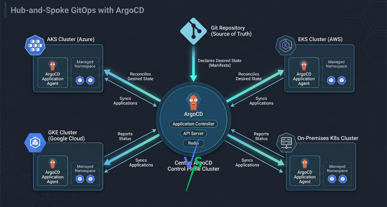
GitOps Beyond ArgoCD: Patterns That Scale for Large Engineering Organisations
ArgoCD became the default answer when someone said "GitOps" for a good few years. It solved the most common problem neatly: sync your Kubernetes...
-

From Prototype to Production: The Engineering Checklist That Actually Matters
Prototypes lie. They perform well in demos because they are not doing any of the work that production systems actually do. There is no...
-
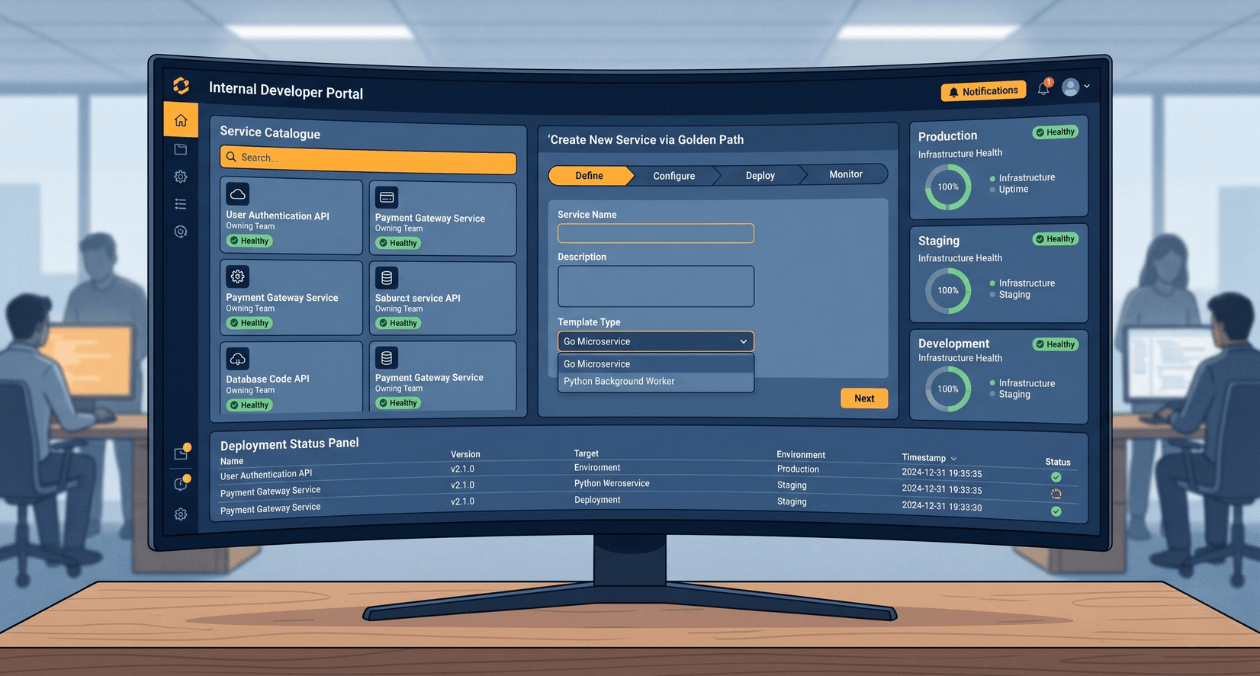
Building a Developer Experience (DX) Platform: From Golden Paths to Self-Service Infrastructure
There is a measurement problem at the heart of platform engineering. The people who benefit most from a well-built internal developer platform are often...
GitOps Beyond ArgoCD: Patterns That Scale for Large Engineering Organisations
ArgoCD became the default answer when someone said "GitOps" for a good few years. It solved the most common problem neatly: sync your Kubernetes...
From Prototype to Production: The Engineering Checklist That Actually Matters
Prototypes lie. They perform well in demos because they are not doing any of the work that production systems actually do. There is no...
Building a Developer Experience (DX) Platform: From Golden Paths to Self-Service Infrastructure
There is a measurement problem at the heart of platform engineering. The people who benefit most from a well-built internal developer platform are often...