

TABLE OF CONTENTS
Building Observable Systems: Metrics, Logs, Traces, and the Modern Monitoring Stack

Production systems fail in ways that surprise even the engineers who built them. A query that ran in 4 milliseconds in staging takes 3 seconds under real load. A microservice that looks healthy in isolation silently corrupts data when its upstream dependency degrades. A memory leak that does not trigger alerts for six hours finally takes down a critical API at 3:00 AM.
These failures share a common root cause: the system was not observable. The engineers had no clear window into what the software was actually doing in production. They had monitoring, perhaps, but monitoring that told them something broke is not the same as observability that shows them why it broke, where it started, and which path through the system the failure traveled.
Observability has matured from a theoretical concept borrowed from control engineering into a concrete engineering discipline with well-defined practices, established tooling, and measurable organizational outcomes. This guide walks through the three fundamental pillars of observability, the architectural decisions that shape your monitoring stack, and the operational patterns that separate teams who detect problems early from teams who learn about them from customers.
The Observability vs. Monitoring Distinction
Monitoring and observability are related but they are not the same thing. The distinction matters because it changes how you instrument your systems and how your teams respond to production incidents.
Monitoring answers the question: is the system healthy? It tracks predefined conditions against thresholds. CPU above 80%? Send an alert. Error rate above 1%? Page the on-call engineer. Monitoring is effective when you already know which failure modes are possible, because you have explicitly defined the conditions you want to watch for.
Observability answers a different question: what is the system doing and why? It captures rich enough telemetry data that engineers can ask arbitrary questions about system behavior after a failure occurs, including questions they could not have anticipated before the failure. A truly observable system allows you to understand novel failure modes, not just the ones your monitoring was configured to detect.
The practical implication: monitoring without observability leaves gaps. You will receive an alert that latency has spiked, but without traces you cannot determine which service in your call chain introduced the spike. You will see elevated error rates in your metrics, but without structured logs you cannot identify which subset of requests failed and what they had in common. Observability gives monitoring its diagnostic depth.
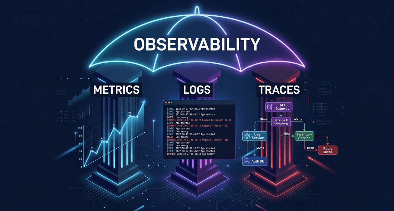
The Three Pillars: Metrics, Logs, and Traces
Metrics: The Quantitative Health Signal
Metrics are numerical measurements sampled over time. They answer quantitative questions: how many requests per second is this service handling? What is the 95th percentile response time for the checkout endpoint? How much memory is the application consuming right now?
Metrics are the most storage-efficient form of telemetry because they aggregate data into numerical summaries. A counter that increments with every HTTP request carries far less storage overhead than a log line for every request. This efficiency makes metrics the right tool for long-term trend analysis, capacity planning, and real-time alerting dashboards.
Prometheus has become the de facto standard for metrics collection in cloud-native environments. It uses a pull-based model where the Prometheus server scrapes /metrics endpoints exposed by instrumented applications at configurable intervals. The Prometheus data model identifies every metric by a name and a set of labels that provide dimensional context.
| Metric Type | Definition | Example Use Case |
|---|---|---|
| Counter | Monotonically increasing value, never decreases | Total HTTP requests served |
| Gauge | Value that can increase or decrease | Current active database connections |
| Histogram | Samples observations into configurable buckets | Request duration distribution (p50, p95, p99) |
| Summary | Streaming calculation of quantiles over a sliding window | Client-side latency percentile calculation |
The RED Method for Service Metrics
Tom Wilkie at Grafana Labs formalized the RED method as a practical framework for what metrics to capture for every service in a microservices architecture.
| Signal | What to Measure |
|---|---|
| Rate | Number of requests per second the service is handling |
| Errors | Number of requests per second that are failing |
| Duration | Distribution of time each request takes |
RED aligns closely with the Four Golden Signals from Google SRE (latency, traffic, errors, saturation) and gives teams a concrete starting point for instrumenting new services. A service that exposes RED metrics immediately provides enough telemetry to build a meaningful health dashboard and configure meaningful alerts.
Logs: The Narrative Record
Logs are timestamped records of discrete events that occurred within the system. Where metrics tell you that error rate increased, logs tell you exactly which requests failed, what error messages they produced, which user triggered them, and what the system state was at the moment of failure.
Unstructured logs, plain text lines written by application code, are the legacy format that most systems still produce. They are human-readable but machine-unfriendly. Querying unstructured logs requires regex pattern matching, which is brittle, slow at scale, and impossible to aggregate meaningfully.
Structured logging replaces free-text output with consistently formatted records, typically JSON, where every field has a defined key and machine-readable value. Structured logs enable filtering, aggregation, and correlation that unstructured logs simply cannot support at production volumes.
Log aggregation platforms collect structured logs from all services in a distributed system and index them for fast search and analysis. The dominant open-source stack pairs Loki (from Grafana Labs) with Grafana for visualization. Commercial alternatives include Datadog Log Management, Elastic (ELK stack), and Splunk.
| Platform | Approach | Best Fit For |
|---|---|---|
| Loki + Grafana | Label-based indexing, low cost, Prometheus-aligned | Teams already running Prometheus/Grafana |
| Elastic (ELK) | Full-text inverted index, powerful querying | High-volume search, complex analytics |
| Datadog Logs | Managed SaaS, deep APM integration | Teams with budget for managed observability |
| Splunk | Enterprise-grade SIEM and log intelligence | Security and compliance-heavy environments |
Log Sampling and Cost Management
High-throughput services can generate billions of log lines per day. Storing all of them is expensive and often unnecessary. Tail-based sampling logs 100% of error events and a configurable percentage of successful requests, capturing full fidelity where it matters while reducing storage costs for routine traffic.
Vector and Fluent Bit are lightweight log shippers that run as sidecar containers or DaemonSets in Kubernetes environments. They handle log collection, transformation, sampling, and routing before logs reach the central storage backend, removing per-record cost at the source rather than paying to store data and then discard it.
Distributed Traces: Following Requests Across Services
Distributed tracing tracks a single request as it propagates through multiple services in a microservices architecture. Each unit of work within that request generates a span. Spans carry a shared trace ID that binds them together into a complete picture of the request’s journey.
A trace for a user checkout request in an e-commerce system might include spans from the API gateway, the authentication service, the product catalog service, the inventory service, the pricing engine, the payment processor, and the order database. When checkout latency spikes, the trace shows exactly which span in that sequence regressed and by how much.
OpenTelemetry (OTel) is the CNCF-backed open standard for distributed tracing instrumentation. It provides vendor-neutral SDKs for over a dozen languages that instrument application code once and export traces to any compatible backend. Teams that adopt OpenTelemetry avoid vendor lock-in because their instrumentation works with Jaeger, Zipkin, Honeycomb, Datadog, and any other OTel-compatible backend.
| OTel Concept | Definition |
|---|---|
| Span | Single unit of work with name, start/end time, status, and attributes |
| Trace | Collection of spans sharing a trace ID, representing one end-to-end request |
| Context Propagation | Mechanism for passing trace ID and span ID across service boundaries via headers |
| Exporter | Component that sends telemetry data to a specific backend (Jaeger, Datadog, etc.) |
| Collector | OTel Collector: receives, processes, and routes telemetry from multiple sources |
Instrument Your Systems for Full Observability
The Modern Monitoring Stack: Architecture Patterns
The Grafana Observability Stack
Grafana Labs has assembled the most widely adopted open-source observability stack by building tools designed to work together while remaining independently useful.
| Component | Role | Data Type |
|---|---|---|
| Prometheus | Metrics collection and storage | Time-series metrics |
| Loki | Log aggregation and querying | Structured and unstructured logs |
| Tempo | Distributed trace storage | Trace spans via OTel or Jaeger protocol |
| Grafana | Unified visualization and alerting | All three signal types |
| Mimir | Long-term scalable Prometheus storage | High-cardinality metrics at scale |
The integration between these tools is what makes the stack powerful. Grafana dashboards can correlate metrics, logs, and traces in a single view. An alert fired by Prometheus can deep-link directly to the Loki logs and Tempo traces that are time-correlated with the alert window, compressing the distance between detection and diagnosis.
Managed Observability Platforms
Self-hosting the Grafana stack requires operational capacity to manage the storage backends, retention policies, and scaling of the observability infrastructure itself. For many engineering teams, managed SaaS platforms offer a better trade-off.
| Platform | Strengths | Typical Use Case |
|---|---|---|
| Datadog | Deep APM, infrastructure correlation, ML-based anomaly detection | Large engineering orgs with budget for full observability |
| Honeycomb | High-cardinality event exploration, BubbleUp analysis | Teams doing deep trace-driven debugging |
| New Relic | Full-stack observability, code-level profiling | Application performance monitoring focus |
| Dynatrace | AI-powered root cause analysis, automatic discovery | Enterprise environments with complex topology |
OpenTelemetry Collector as the Central Routing Layer
The OpenTelemetry Collector acts as a vendor-neutral telemetry pipeline that sits between instrumented applications and backend storage. Rather than configuring each application to send data directly to a specific backend, applications export telemetry to the local OTel Collector, which handles routing, batching, sampling, and transformation.
This architecture provides backend portability. When your organization decides to switch from Jaeger to Tempo for trace storage, you change one configuration in the Collector rather than modifying instrumentation code in every service. It also enables fanout: the same trace can be sent to both a local Jaeger instance for development and a Honeycomb cloud account for production analysis.
Alerting Architecture and Alert Quality
The Alert Quality Problem
Poorly designed alerting is one of the most damaging patterns in production operations. When every dashboard has too many alert rules, and every minor fluctuation pages the on-call engineer, the on-call rotation becomes a constant source of stress that degrades response quality. Alert fatigue is a documented phenomenon that leads to engineers dismissing or ignoring alerts, including the ones that matter.
High-quality alerting follows two principles. First, every alert should be actionable: receiving it should tell the engineer exactly what to investigate and produce a decision within a defined time window. Second, alerts should be symptom-based rather than cause-based. Alerting on user-visible symptoms (elevated error rate, increased latency at the 99th percentile) rather than potential causes (CPU above 70%) produces fewer false positives and more meaningful signals.
Alerting Tiers
| Tier | Condition | Response |
|---|---|---|
| Page (Critical) | User-facing SLO breach or imminent breach | Immediate on-call wake-up, incident declared |
| Ticket (Warning) | Trend indicating future SLO risk within hours | Next-business-day investigation, no page |
| Dashboard Only | Informational signal, no action required | Visible in dashboards, no notification generated |
Robustness requirements for critical alerts: they must have a minimum 5-minute evaluation window to prevent single-datapoint spikes from triggering pages. They must have a clear runbook linked in the alert body. And they must be reviewed quarterly to confirm they still reflect the current system architecture and remain actionable.
SLO-Based Alerting with Error Budgets
Service Level Objectives (SLOs) define the target reliability that a service promises to its consumers. An SLO of 99.9% availability over a 30-day window means the service is allowed approximately 43 minutes of cumulative downtime per month. That allowance is the error budget.
Error budget burn rate alerting fires when the rate of budget consumption indicates the full budget will be exhausted before the end of the window. A burn rate of 14.4x over a one-hour window means the service is consuming 30 days of error budget in just two hours. This condition warrants an immediate page even if the absolute error rate looks modest.
Google’s SRE Workbook, freely available at sre.google/workbook, provides detailed multi-window burn rate alerting formulas that balance fast detection against low false-positive rates. This SLO alerting approach is implemented natively in Prometheus Alertmanager through recording rules and alert expressions.
Instrument Your Systems for Full Observability
Instrumentation Strategies for Application Code
Auto-Instrumentation vs. Manual Instrumentation
OpenTelemetry provides auto-instrumentation libraries for popular frameworks that capture traces, metrics, and logs automatically without requiring developers to modify application code. For Node.js applications, the @opentelemetry/auto-instrumentations-node package instruments Express, HTTP, gRPC, database clients, and Redis clients automatically at startup.
Auto-instrumentation captures framework-level operations but does not understand business logic. It will trace a database query but will not attribute that query to a specific user workflow or business transaction. Manual instrumentation adds custom spans and attributes that carry business context: the user ID, the order value, the product category, the experiment cohort. This business-layer instrumentation is what elevates traces from debugging tools into product analytics instruments.
| Instrumentation Type | What It Captures |
|---|---|
| Auto-instrumentation | HTTP calls, DB queries, cache operations, framework lifecycle events |
| Manual spans | Business transactions, custom operations, domain-specific context |
| Custom metrics | Business KPIs: order rate, payment success rate, search conversion |
| Structured log fields | User ID, session ID, feature flag state, A/B test cohort |
The Trace Context as the Correlation Key
The trace ID is the most powerful correlating key in an observable system. When your structured logs include the trace ID as a field on every log line, and your metrics include it as a label on relevant measurements, you can navigate seamlessly from a metric alert to the correlated traces and from those traces to the specific log lines emitted during the failing spans.
Grafana’s Explore view supports exactly this navigation pattern. Click a spike in your error rate Prometheus graph, jump to Loki to see the log lines from that time window, then click the trace ID in a log line to open the corresponding Tempo trace. This three-signal correlation workflow compresses incident diagnosis time from hours of grep-based log archaeology to minutes of guided navigation through correlated telemetry.
Kubernetes-Native Observability
kube-state-metrics and node-exporter
Kubernetes exposes two essential observability surfaces. kube-state-metrics translates Kubernetes object state (Deployment replicas, Pod status, Job completion, HPA scale events) into Prometheus metrics. node-exporter exposes host-level metrics (CPU, memory, disk I/O, network throughput) for each cluster node.
These two exporters together with the kubelet /metrics endpoint provide the foundational infrastructure visibility layer. The kube-prometheus-stack Helm chart bundles Prometheus, Alertmanager, Grafana, kube-state-metrics, and node-exporter into a single installation with pre-configured dashboards and alert rules maintained by the community.
Service Mesh Observability
Service meshes like Istio and Linkerd inject sidecar proxies into every Pod that intercept all inbound and outbound network traffic. These proxies generate telemetry for every service-to-service request without any application-level instrumentation: request count, response latency, error rate, and bytes transferred.
The result is a network-level observability layer that works uniformly across all services regardless of their programming language or framework. In polyglot microservices architectures where some services use Java, some Python, and some Go, service mesh telemetry provides a consistent baseline visibility layer before any language-specific instrumentation is applied.
Connecting Observability to Deployment Safety
Observability is not only a production incident tool. It is the safety mechanism that makes progressive delivery viable. Canary releases and Blue-Green deployments, both covered in the March 17 article on zero-downtime deployment strategies, depend on your observability stack to provide the health signals that automated promotion decisions evaluate.
Argo Rollouts integrates with Prometheus through its Analysis Run mechanism. An AnalysisTemplate defines which Prometheus queries to evaluate, what thresholds constitute a healthy canary, and how long to observe before promoting to the next traffic percentage. Without a mature metrics layer, automated canary analysis cannot function. The observability stack is the prerequisite for automated deployment safety.
| Deployment Phase | Observability Signal Used | Action Taken |
|---|---|---|
| Pre-switch validation | Synthetic test metrics against Green environment | Proceed or abort before any user traffic shifts |
| Canary promotion gate | RED metrics comparison: canary vs. stable baseline | Advance to next traffic percentage or rollback |
| Post-deployment validation | SLO burn rate over 30-minute window | Confirm release or trigger rollback |
| Ongoing production health | Error budget consumption rate | Inform next release decision and deployment frequency |
Instrument Your Systems for Full Observability
Profiling: The Fourth Pillar
Continuous profiling is increasingly recognized as a fourth observability signal alongside metrics, logs, and traces. Where traces show which service in the call chain is slow, profiling shows which function within that service is consuming the most CPU time or allocating the most memory.
Tools like Pyroscope (now part of Grafana) and Parca provide always-on continuous profiling that samples application stack traces at low overhead, typically under 1% CPU overhead. Profiling data attached to a trace span answers the question that traces cannot: within the 200-millisecond span attributed to the payment service, which specific code path consumed the time?
Continuous profiling integrates into incident response by correlating profiles with the same trace IDs used by distributed tracing. When investigating a latency regression, an engineer navigates from the metric alert to the trace to the correlated CPU profile, completing the full diagnostic chain from symptom to root cause without leaving their observability tooling.
Building a Maturity Model for Observability
Most engineering teams do not achieve full observability overnight. It develops incrementally across a maturity progression that aligns investment with organizational scale and reliability requirements.
| Maturity Level | Characteristics | Key Tools |
|---|---|---|
| Level 1: Basic Monitoring | Health checks, uptime monitoring, basic CPU/memory alerts | CloudWatch, UptimeRobot, basic Grafana |
| Level 2: Metrics and Logs | RED metrics per service, structured logging, centralized log search | Prometheus, Grafana, Loki or ELK |
| Level 3: Distributed Tracing | End-to-end traces across all services, OTel instrumentation | Tempo or Jaeger, OTel Collector |
| Level 4: SLO-Driven | Defined SLOs, error budget tracking, burn rate alerting | Prometheus recording rules, Alertmanager |
| Level 5: Continuous Profiling | Always-on CPU and memory profiling correlated with traces | Pyroscope, Parca, Grafana Profiles |
Most production engineering teams operating at scale should target Level 4 as their baseline. Level 5 profiling is particularly valuable for performance-critical services and large monolithic applications where trace-level granularity is insufficient for identifying hot paths.
Practical Implementation Path
The sequence in which you build out your observability stack matters. Starting with distributed tracing before you have basic metrics in place is a common mistake that results in a sophisticated tracing setup without the aggregated health signals needed for alerting.
A pragmatic implementation sequence follows four phases. In the first phase, deploy the kube-prometheus-stack to establish cluster-level metrics and a functional Grafana instance with pre-built Kubernetes dashboards. Define RED metrics for your two or three highest-traffic services and configure paging alerts based on error rate and latency thresholds.
In the second phase, introduce structured logging and centralize logs in Loki or your chosen backend. Add trace ID fields to all log output. This prepares the correlation layer before tracing is introduced.
In the third phase, deploy the OTel Collector and begin instrumenting services with auto-instrumentation libraries. Integrate Tempo for trace storage and configure Grafana data source links between metrics, logs, and traces.
In the fourth phase, define formal SLOs for user-facing services, implement error budget recording rules, and configure multi-window burn rate alerts. Review and eliminate alert rules that are not actionable or that have fired without producing meaningful incidents in the prior 90 days.
The full-stack engineering services available through Askan Technologies cover each of these implementation phases, from initial infrastructure setup through instrumentation, dashboard design, and ongoing SRE consulting for teams building toward higher maturity levels.
SEO Meta Information
| SEO Field | Value |
|---|---|
| SEO Title | Modern Observability Guide: Making Sense of Metrics, Logs, and Traces |
| URL Slug | /observability-engineering-metrics-logs-traces-monitoring-stack/ |
| Meta Description | Learn how to build observable systems using metrics, logs, and distributed traces. Covers Prometheus, OpenTelemetry, Grafana stack, SLO-based alerting, and Kubernetes observability for SREs and DevOps engineers. |
| Primary Keyword | observability engineering |
| Secondary Keywords | monitoring, logging, distributed tracing, metrics, SRE practices, Prometheus, OpenTelemetry, Grafana |
| Content Type | Technical Deep Dive |
| Target Audience | SREs, DevOps Engineers, Platform Teams |
| Category | DevOps & Automation |
Most popular pages

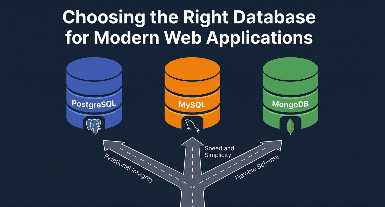
PostgreSQL vs MySQL vs MongoDB: Database Selection for Modern Web Applications
The database you choose for a web application is one of the most consequential architectural decisions your team will make. Unlike a framework or...
-
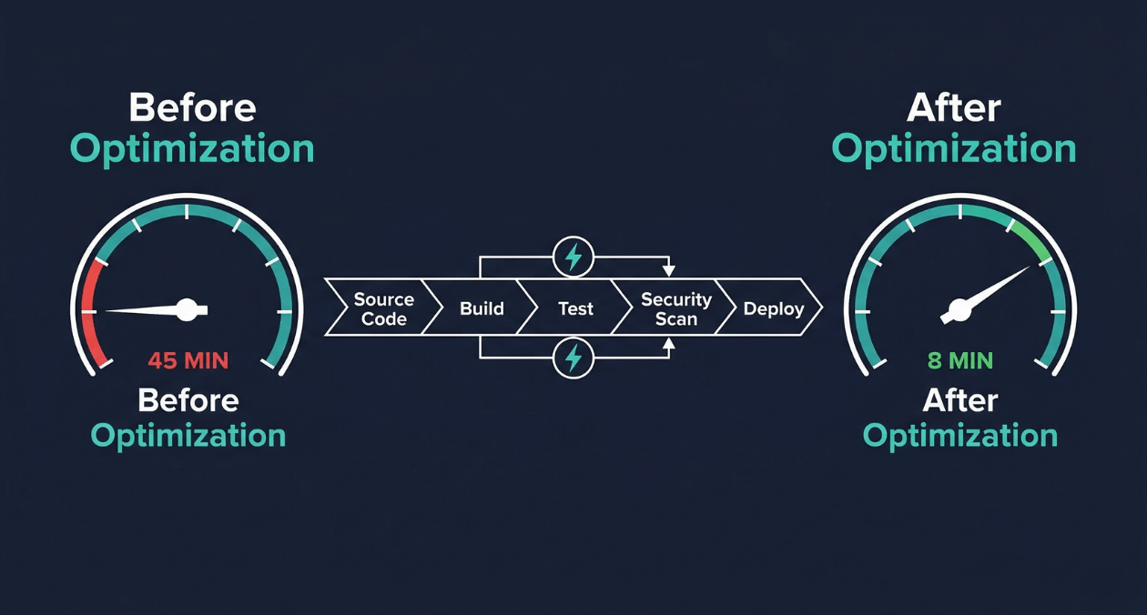
CI/CD Pipeline Optimization: Reducing Build Times from 45 Minutes to 8 Minutes
A 45-minute build pipeline is not just a productivity inconvenience. It is a structural constraint on how your engineering organization operates. When every commit...
-
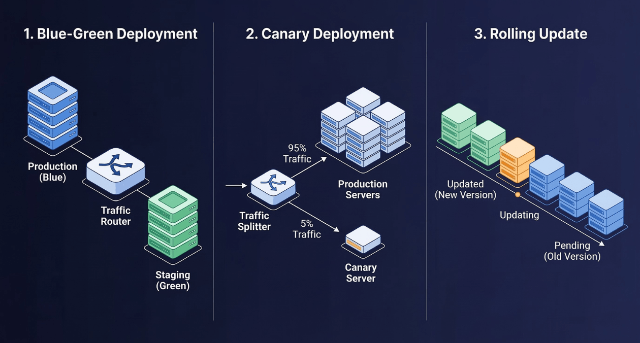
Zero-Downtime Deployment Strategies: Blue-Green, Canary, and Rolling Updates Compared
Every minute of unplanned downtime carries a measurable cost. For enterprise SaaS platforms, that cost routinely exceeds tens of thousands of dollars per incident....
PostgreSQL vs MySQL vs MongoDB: Database Selection for Modern Web Applications
The database you choose for a web application is one of the most consequential architectural decisions your team will make. Unlike a framework or...
CI/CD Pipeline Optimization: Reducing Build Times from 45 Minutes to 8 Minutes
A 45-minute build pipeline is not just a productivity inconvenience. It is a structural constraint on how your engineering organization operates. When every commit...
Zero-Downtime Deployment Strategies: Blue-Green, Canary, and Rolling Updates Compared
Every minute of unplanned downtime carries a measurable cost. For enterprise SaaS platforms, that cost routinely exceeds tens of thousands of dollars per incident....